LAB 7 - MAE4190 FAST ROBOTS

Welcome to lab 7 of fast robots! In this lab we will be implementing the Kalman filter on our car controls.

Lab Tasks

In order to implement a Kalman Filter, we will first be needing a state space model of the car.

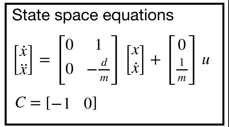
To get the estimates for our A and B matrices, we will therefore need the car’s drag and momentum.

1. Testing for Drag and Momentum

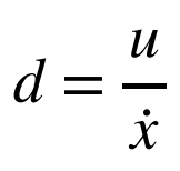
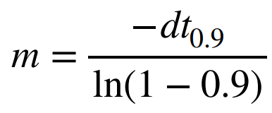
Using a step response and giving the motors a constant input, I obtained ToF sensor data with which I calculated velocity to plot against time. From the plots I obtained the steady state velocity and 90% rise time for the d and m calculations:

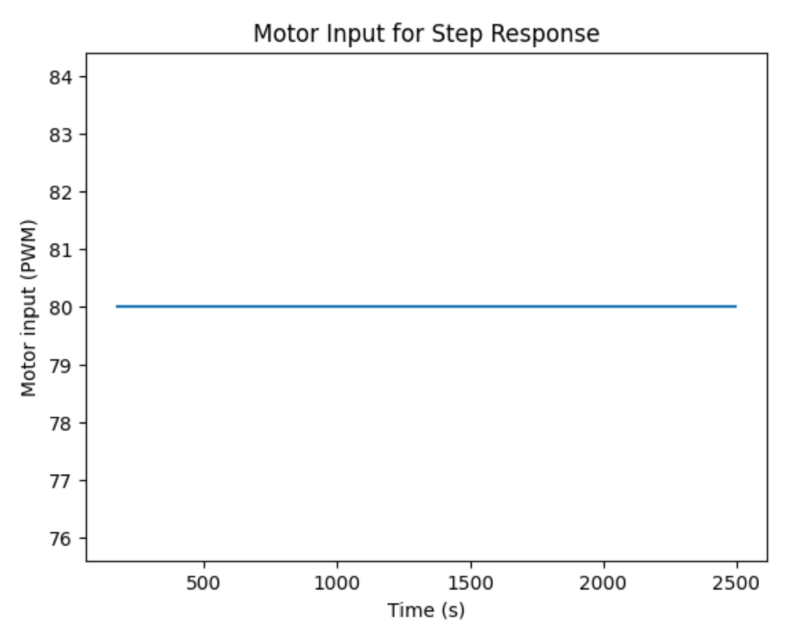
I chose the step response input to be 80 (and the calibrated speed 112); to be of similar size to the PWM value you used in Lab 5 (to keep the dynamics similar). Pick something between 50%-100% of the maximum u.

placed car 3m from wall –> far enough to reach steady state, but close enough so that tof sensor does not lose range (still could be a bit farther as it still hit the wall before fully reaching stable steady state) active braking

            while (time_interval < step_time) {
                time_interval = millis() - start_time;

                //tof sensor
                if (distanceSensor2.checkForDataReady()){
                    drag_dis = distanceSensor2.getDistance();
                    distanceSensor2.clearInterrupt();
                    distance_doc[tindex] = drag_dis;
                    time_doc[tindex] = millis() - start_time;
                    tindex++;
                }

                //active braking
                if (drag_dis < target_dis) {
                    control_stop();
                    return;
                }

                //drive forwards
                analogWrite(MOTOR1PIN1, step_speed);
                analogWrite(MOTOR2PIN1, step_speed * 1.4);
                analogWrite(MOTOR1PIN2, 0);
                analogWrite(MOTOR2PIN2, 0);

            }

            control_stop();
            delay(1000);
            distanceSensor2.stopRanging();

Decided to save my data with a csv file so that my data is not lost when the kernel resets

To calculate the velocity I changed the stored data into numpy arrays for easier calcs.

dd = np.diff(dist_array)
dt = np.diff(time_array)
vel_array = - dd / dt

since the distance reading becomes smaller, the np.diff returns negative numbers and hence the added sign during the velocity calculation.

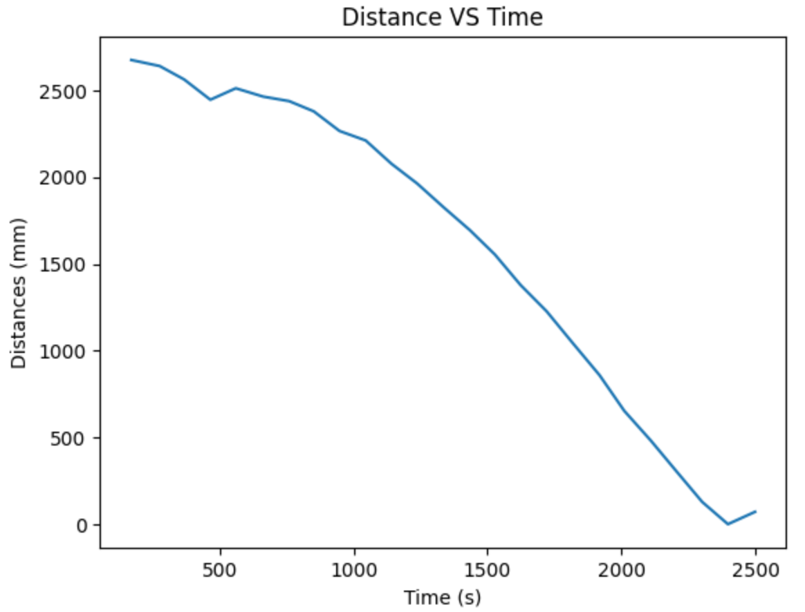
VELOCITY OUTPUT –> plotted in desmos from raw data to curve fit and find variables from fitted graph equation

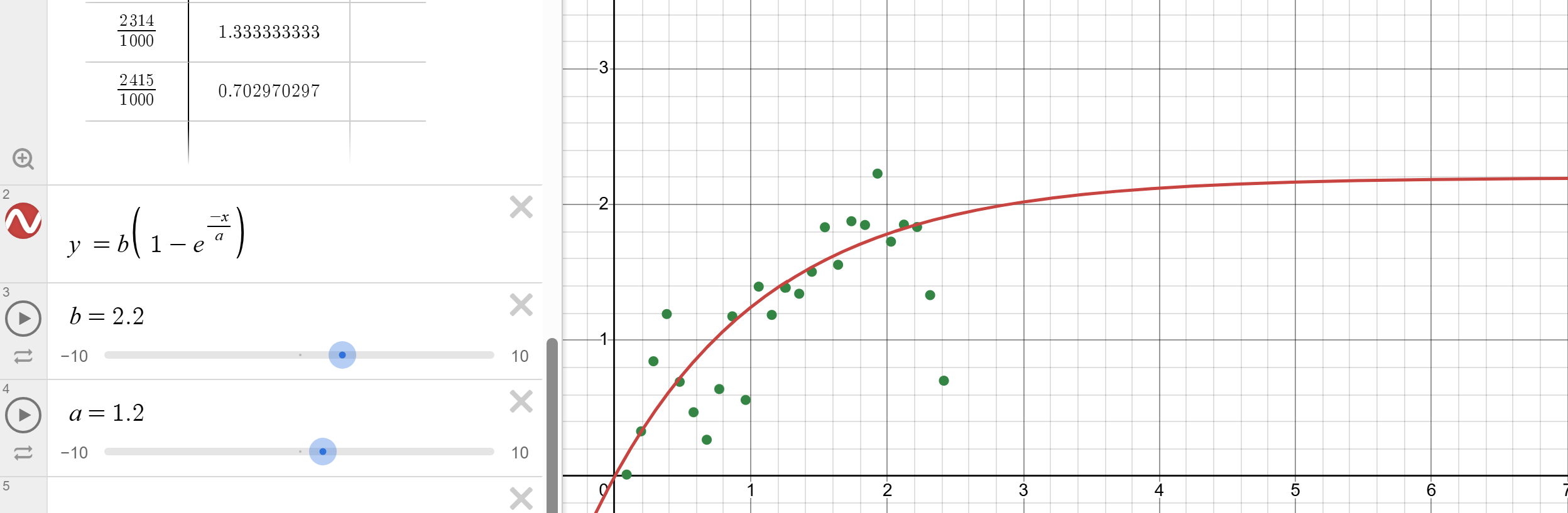
Fitted exponential curve

b = 2.2 is my steady state velocity a = 1.2 is the tau, the time constant

To find the 90% rise time, I found the point at which velocity reaches 1.98 m/s, which is about 2.763s.

With this obtained data, I calculated the following for my matrices:

\[d = \frac{u}{dx} = 0.036364\] \[m = \frac{- d \cdot t(0.9)}{\ln(0.1)} = 0.043635\]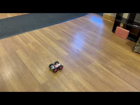

2. Initialize KF

My sampling rate: According to previous tests of the ToF sampling rate, it’s on average about in 100ms intervals. The Delta_t should be 0.1 then.

Matrix explanation + discretization

d = 0.036364
m = 0.043635
Delta_t = 0.1
#dimensions of state space
n = 2

A = np.array([[0, 1], [0, d/m]])
B = np.array([[0], [1/m]])

Ad = np.eye(n) + Delta_t * A
Bd = Delta_t * B

C state explanation

C = np.array([[-1,0]])

initializing state vector:

TOF = np.array(dist_array)
x = np.array([[-TOF[0]],[0]])

initialize process noise and sensor noise covariance matrices

I started off with the equations for the position, velocity and measurement uncertainty shown in lecture:

\[\begin{aligned} \sigma_1 &= \sqrt{10^2 \cdot \frac{1}{\Delta T}} = 31.6 \\ \sigma_2 &= \sqrt{10^2 \cdot \frac{1}{\Delta T}} = 31.6 \\ \sigma_3 &= 20 \end{aligned}\]

Sigma3 which determines how much the measurements are trusted against model predictions, was tweaked later with trial and error.

sig_u=np.array([[sigma_1**2,0],[0,sigma_2**2]])
sig_z=np.array([[sigma_3**2]])

3. Testing Kalman Filter in Python

def kf(mu,sigma,u,y):
    
    mu_p = Ad.dot(mu) + Bd.dot(u) 
    sigma_p = Ad.dot(sigma.dot(Ad.transpose())) + sig_u
    
    sigma_m = C.dot(sigma_p.dot(C.transpose())) + sig_z
    kkf_gain = sigma_p.dot(C.transpose().dot(np.linalg.inv(sigma_m)))

    y_m = y-C.dot(mu_p)
    mu = mu_p + kkf_gain.dot(y_m)    
    sigma=(np.eye(2)-kkf_gain.dot(C)).dot(sigma_p)

    return mu,sigma

TOF = np.array(dist_array)
x = np.array([[TOF[0]],[0]])
sigma = np.eye(n)
dist_kf = []
 
for i in range(len(dist_array)):
    x, sigma = kf(x, sigma, u_ss, dist_array[i])
    dist_kf.append(x[0, 0])

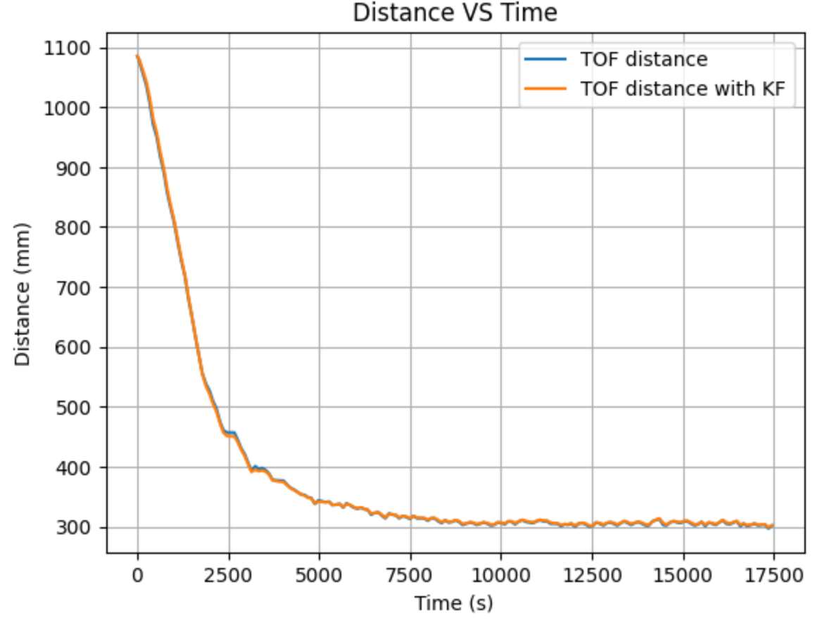
Turns out, having the sigma3 be around 20 was already a pretty good estimate. The Kalman filter followed the raw data pretty closely. However, as I increased it to 50 and 70 respectively below:

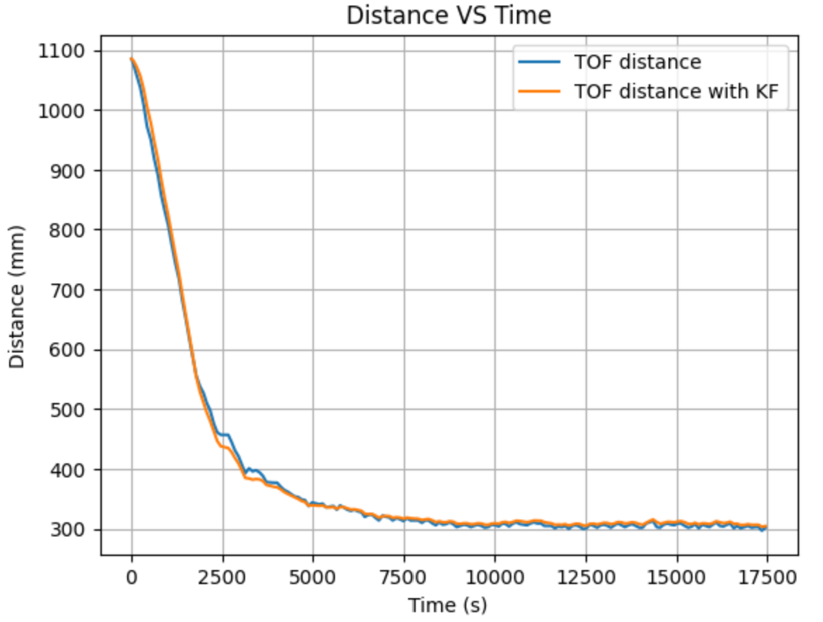
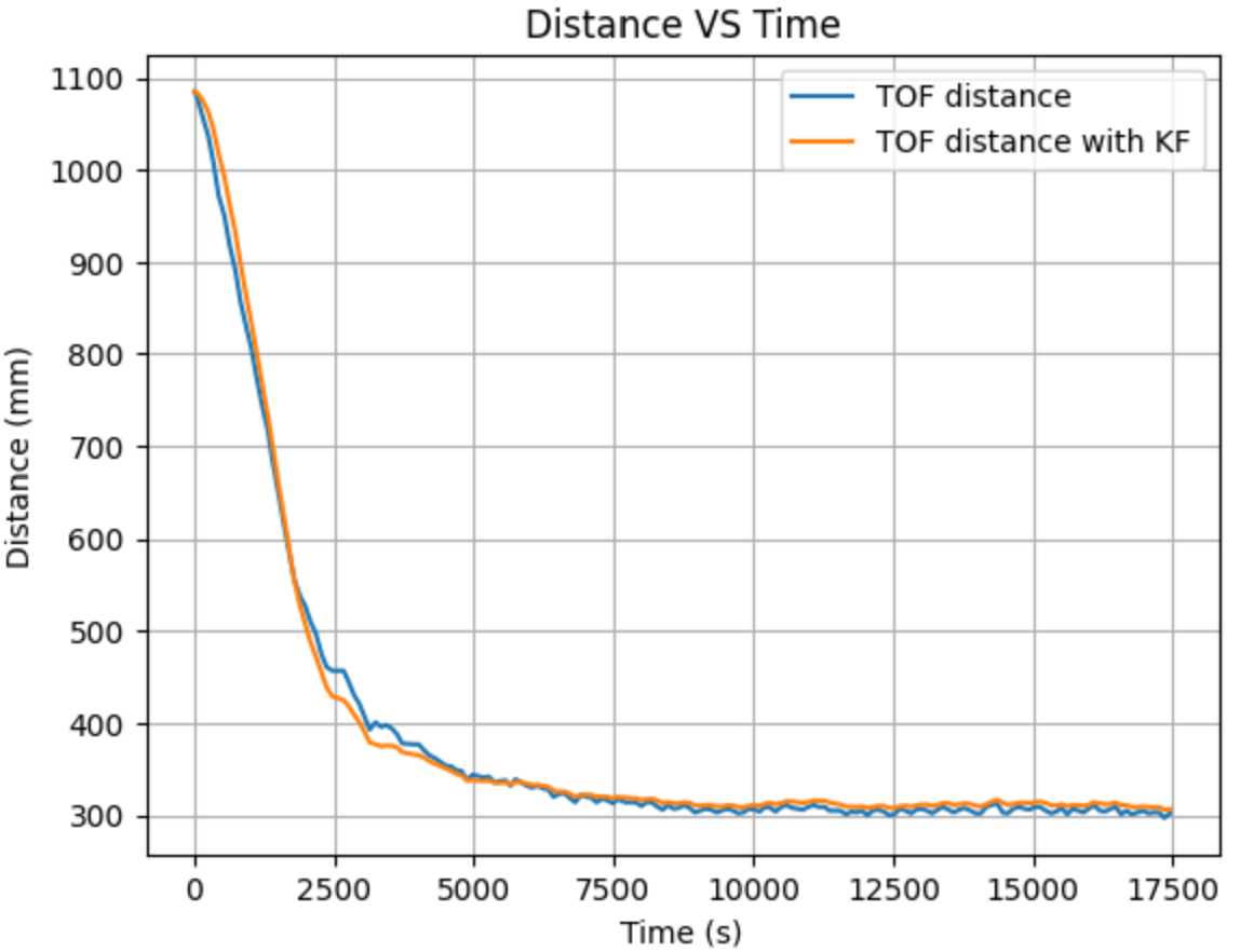
(see if I can put a caption on these and put them side by side)

The filter begins to have a bigger and bigger mismatch as compared to the raw data, while it becomes smoother with less effects from the sensor noise. I decided in the end to have sigma3 be 30 to get a smooth enough prediction without straying from the raw data too much.

4. Implementing KF on the Robot

initializing matrices

KF function implementing into my PID function (does my funky PID function work with KF)

oops so turns out the KF was actually smoothing out the data a little too much, the distance vs time graphs show a substantial offset from the actual measurements. The Kalman filter lags behind and ends up estimating that we are farther from the wall than reality, so my car would sometimes run into the wall. I dialed it back to around 26

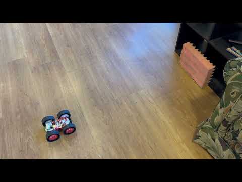
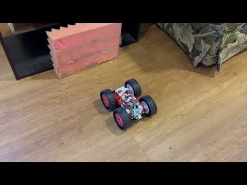
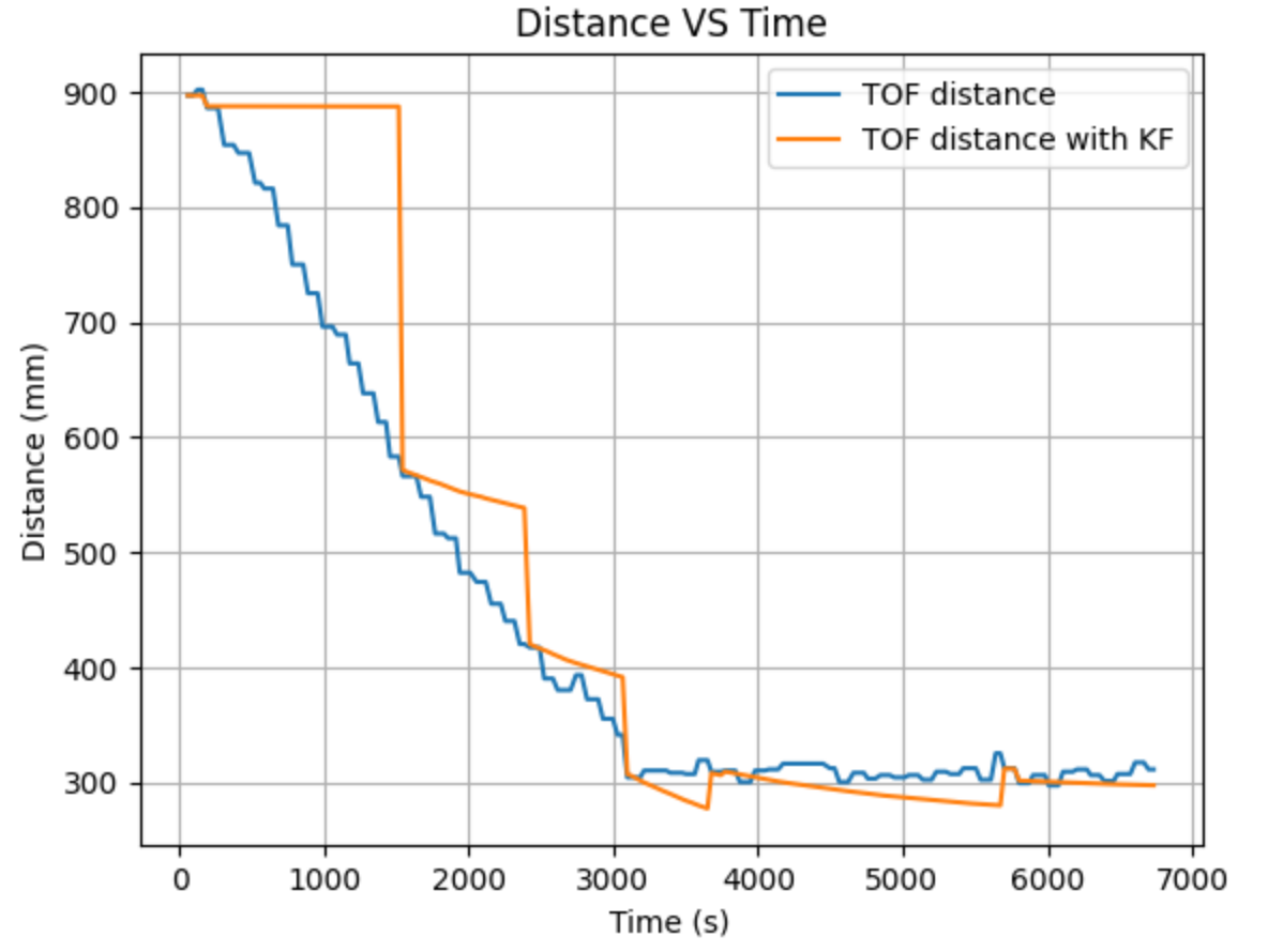
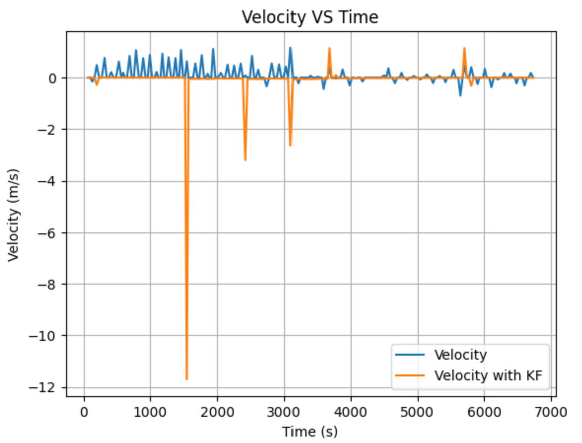
the kalman filter was overall quite successful on my robot, the adjustment speed improved a lot (lab 5 was quite slow in small adjustments) and the robot responds faster